
Available on Bioconductor
Read the paper in Briefings in Bioinformatics
What is TaxSEA?
TaxSEA is technique to move from analysisng individual microbes to looking at groups of microbes with a shared functional characteristic.
Traditional microbiome analysis tools often look at individual microbes going up or down. This sounds sensible but in human microbiome studies it can fail apart because everyone’s microbiome is unique, with few species shared across people.
TaxSEA doesn’t test for individual species but rather asks if there a group of species with a shared characteristic that is altered between groups of people. For example are we seeing a shift in bugs with increased oxygen tolerance, or an increase in bugs which produce a certain metabolite or enzyme, or even are we seeing a change in bugs which have a known disease association in humans. If you want to know more check out our paper, but we find this approach to be far more reproducible than standard Differential Abundance (DA) analysis as well as capable of extracting biologically meaningful patterns. TaxSEA usually can run within seconds with standard hardware.
TaxSEA supports three complementary analysis modes:
- Enrichment using public reference databases
-
ORA – Over-Representation Analysis
- Enrichment using taxonomic sets
Modes 1 and 2 Both use the same taxon-set databases but answer slightly different questions. Mode 1 which is the default we reccomend in most cases takes as input a list of bacteria a rank (E.g. fold change). It then tests whether any of the taxon sets in the database are skewed to one end of the distribution or another. Mode 2 uses the same database but only takes as input a list of bacterial names. While answering a similar question this approach is often less powerful as it requires a hard cut-off to select bacteria of interest.
Mode 3 allows users to test for differences at a particular taxonomic rank. For example instead of just summing up or aggregating all the species in a genus. We see if the distribution of species within a genus is different between groups. This is a more powerful approach as simply summing/aggregating to a rank can risk missing when you can get shifts within a taxon. This approach is implemented in the taxon_set_ranks() function.
In short, TaxSEA aims to make it easy to intepret changes in your microbiome data.
TaxSEA takes as input a vector of species names and a rank. For example log2 fold changes or Spearman’s rho.
Note: Although TaxSEA in principle can be applied to microbiome data from any source, the databases utilized largely cover human associated microbiomes and the human gut microbiome in particular. As such the database testing in TaxSEA will likely perform best on human gut microbiome data.
Taxon set database
By default TaxSEA utilizes taxon sets generated from six reference databases (BacDive,gutMGene, GMrepo v2, MiMeDB, mBodyMap, BugSigDB). See below for examples of using custom databases or taxonomically defined taxon sets.
Please cite the appropriate database if using:
- Schober et al. BacDive in 2025: the core database for prokaryotic strain data. Nucleic Acids Res. 2025.
- Cheng et al. gutMGene: a comprehensive database for target genes of gut microbes and microbial metabolites. Nucleic Acids Res. 2022.
- Dai et al. GMrepo v2: a curated human gut microbiome database with special focus on disease markers and cross-dataset comparison Nucleic Acids Res. 2022.
- Wishart et. al. MiMeDB: the Human Microbial Metabolome Database Nucleic Acids Res. 2023.
- Jin et al. mBodyMap: a curated database for microbes across human body and their associations with health and diseases. Nucleic Acids Res. 2022.
- Geistlinger et al. BugSigDB captures patterns of differential abundance across a broad range of host-associated microbial signatures. Nature Biotech. 2023.
Installation
if (!requireNamespace("BiocManager", quietly = TRUE))
    install.packages("BiocManager")
BiocManager::install("TaxSEA")
Usage
Quick start (mode 1, enrichment rank based)
library(TaxSEA)

# Retrieve taxon sets containing Bifidobacterium longum.
blong.sets <- get_taxon_sets(taxon="Bifidobacterium_longum")

# Run TaxSEA with test data provided
data(TaxSEA_test_data)
taxsea_results <- TaxSEA(taxon_ranks=TaxSEA_test_data)

#Enrichments among metabolite producers from gutMgene and MiMeDB
metabolites.df <- taxsea_results$Metabolite_producers

#Enrichments among health and disease signatures from GMRepoV2 and mBodyMap
disease.df <- taxsea_results$Health_associations

#Enrichments among published associations from BugSigDB
bsdb.df <- taxsea_results$BugSigdB
Quick start (mode 2, ORA)
library(TaxSEA)

# A list of oral taxa
test_ORA_input <- c(
  "Streptococcus_mitis",
  "Haemophilus_parainfluenzae",
  "Fusobacterium_periodonticum",
  "Fusobacterium_nucleatum",
  "Neisseria_elongata",
  "Neisseria_flavescens",
  "Streptococcus_sanguinis",
  "Streptococcus_parasanguinis",
  "Streptococcus_salivarius",
  "Capnocytophaga_sputigena"
)


taxsea_results <- TaxSEA(input_taxa=test_ORA_input)

#Enrichments among health and disease signatures from GMRepoV2 and mBodyMap
disease.df <- taxsea_results$Health_associations
Input
TaxSEA supports multiple input types, depending on the analysis mode you choose:
Enrichment mode (rank-based; recommended)
You provide a named numeric vector where:
- The names are taxa (species or genus)
- The values are ranks or signed statistics (e.g. log2 fold changes, correlation coefficients)
In enrichment mode, the input must include all taxa that were tested in your analysis.
Do not apply a significance threshold or pre-filter taxa before running TaxSEA.
The method relies on the full distribution of values to detect coordinated shifts across taxon sets.
ORA mode (set-based)
You provide a character vector of taxa names representing taxa of interest (i.e. a “hit list”).
- No ranking or numeric values are required
- TaxSEA tests whether these taxa are over-represented in predefined taxon sets
- This mode is most appropriate for presence/absence or binary data
Input taxa names should be in the format of like one of the following
- Species name. E.g. “Bifidobacterium longum”, “Bifidobacterium_longum”
- Genus name. E.g. “Bifidobacterium”
- NCBI ID E.g. 216816
#Input IDs with the full taxonomic lineage should be split up. E.g.
x <- "d__Bacteria.p__Actinobacteriota.c__Actinomycetes.o__Bifidobacteriales.f__Bifidobacteriaceae.g__Bifidobacterium"
x <- strsplit(x,split="\\.")[[1]][6]
x <- gsub("g__","",x)

## Running this through a vector of IDs may look something like the following
#new_ids <- sapply(as.character(old_ids),function(y) {strsplit(x = y,split="\\.")[[1]][6]})
#new_ids <- gsub("g__","",new_ids)

## Example test data
library(TaxSEA)
data("TaxSEA_test_data")
head(sample(TaxSEA_test_data),4)
Run TaxSEA with test data
data("TaxSEA_test_data")
taxsea_results <- TaxSEA(taxon_ranks=TaxSEA_test_data)

#Enrichments among metabolite producers from gutMgene and MiMeDB
metabolites.df <- taxsea_results$Metabolite_producers

#Enrichments among health and disease signatures from GMRepoV2 and mBodyMap
disease.df <- taxsea_results$Health_associations

#Enrichments among published associations from BugSigDB
bsdb.df <- taxsea_results$BugSigDB
Test data
The test data provided with TaxSEA consists of log2 fold changes comparing between healthy and IBD. The count data for this was downloaded from curatedMetagenomeData and fold changes generated with LinDA.
- Hall et al. A novel Ruminococcus gnavus clade enriched in inflammatory bowel disease patients** Genome Med. 2017 Nov 28;9(1):103.
- Pasolli et al. Accessible, curated metagenomic data through ExperimentHub. Nat Methods. 2017 Oct 31;14(11):1023-1024. doi: 10.1038/nmeth.4468.
- Zhou et al. LinDA: linear models for differential abundance analysis of microbiome compositional data. Genome Biol. 2022 Apr 14;23(1):95.
Output
The output is a list of three data frames providing enrichment results for metabolite producers, health/disease associations, and published signatures from BugSigDB. Each dataframe has 5 columns
- taxonSetName - The name of the taxon set tested
- median_rank - This is simply the median rank across all detected members in the set. This allows you to see the direction of change
- P value - Kolmogorov-Smirnov test P value.
- FDR - P value adjusted for multiple testing.
- TaxonSet - Returns list of taxa in the set to show what is driving the signal
Custom databases
Many users may want to utilise TaxSEA with a custom database. For example for testing if there is a flag in the TaxSEA function “custom_db” which expects as input a named list of vectors. This is the same format as the default TaxSEA database. Note: using the custom_db flag disables the automatic ID conversion and NCBI API lookup. However we have functionality available via other functions
# Perform enrichment analysis using TaxSEA
custom_taxsea_results <- TaxSEA(taxon_ranks = log2_fold_changes, custom_db = custom_taxon_sets)
custom_taxsea_results <- custom_taxsea_results$custom_sets
Testing for differences in taxonomically defined sets
In addition to taxon sets defined from public databases by, users can define sets based on taxonomy from their own data. We have implemtned this in the taxon_rank_sets() function which takes as input an set of taxa and ranks (similar to enrichment testing above) and then either a table of taxonomic lineage or a TreeSummarizedExperiment object. See below for examples with both approaches.
Current methods to test at higher taxonomic levels (e.g., phylum or family), involve aggregating counts. However, this approach may miss opposing shifts in individual species which cancel each other out, obscuring meaningful biological patterns. For instance, antibiotic treatment may suppress certain species while allowing resistant species within the same genus to expand and occupy the vacant niche, creating an ecological shift that appears as no net change at broader taxonomic levels. Whereas the database testing works best with shotgun metagenomic data in order to have sufficient resolution. This approach is much more widely applicable including to testing with amplicon data such as from 16S rRNA gene sequencing.
#### Enrichment testing with taxonomically defined ranks
# --- Example 1: Data frame input ---
# Create a lineage data frame (e.g., parsed from curatedMetagenomicData)
# The 'species' column must match the names in taxon_ranks.

lineage_df <- data.frame(
  species = c("Cutibacterium_acnes", "Klebsiella_pneumoniae",
              "Propionibacterium_humerusii", "Moraxella_osloensis",
              "Enhydrobacter_aerosaccus", "Staphylococcus_capitis",
              "Staphylococcus_epidermidis", "Staphylococcus_aureus",
              "Escherichia_coli", "Enterobacter_cloacae",
              "Pseudomonas_aeruginosa", "Acinetobacter_baumannii",
              "Lactobacillus_rhamnosus", "Lactobacillus_acidophilus",
              "Bifidobacterium_longum", "Bifidobacterium_breve"),
  kingdom = rep("Bacteria", 16),
  phylum = c("Actinobacteria", "Proteobacteria",
             "Actinobacteria", "Proteobacteria",
             "Proteobacteria", "Firmicutes",
             "Firmicutes", "Firmicutes",
             "Proteobacteria", "Proteobacteria",
             "Proteobacteria", "Proteobacteria",
             "Firmicutes", "Firmicutes",
             "Actinobacteria", "Actinobacteria"),
  class = c("Actinobacteria", "Gammaproteobacteria",
            "Actinobacteria", "Gammaproteobacteria",
            "Alphaproteobacteria", "Bacilli",
            "Bacilli", "Bacilli",
            "Gammaproteobacteria", "Gammaproteobacteria",
            "Gammaproteobacteria", "Gammaproteobacteria",
            "Bacilli", "Bacilli",
            "Actinobacteria", "Actinobacteria"),
  order = c("Propionibacteriales", "Enterobacterales",
            "Propionibacteriales", "Pseudomonadales",
            "Rhodospirillales", "Bacillales",
            "Bacillales", "Bacillales",
            "Enterobacterales", "Enterobacterales",
            "Pseudomonadales", "Pseudomonadales",
            "Lactobacillales", "Lactobacillales",
            "Bifidobacteriales", "Bifidobacteriales"),
  family = c("Propionibacteriaceae", "Enterobacteriaceae",
             "Propionibacteriaceae", "Moraxellaceae",
             "Rhodospirillaceae", "Staphylococcaceae",
             "Staphylococcaceae", "Staphylococcaceae",
             "Enterobacteriaceae", "Enterobacteriaceae",
             "Pseudomonadaceae", "Moraxellaceae",
             "Lactobacillaceae", "Lactobacillaceae",
             "Bifidobacteriaceae", "Bifidobacteriaceae"),
  genus = c("Cutibacterium", "Klebsiella",
            "Cutibacterium", "Moraxella",
            "Enhydrobacter", "Staphylococcus",
            "Staphylococcus", "Staphylococcus",
            "Escherichia", "Enterobacter",
            "Pseudomonas", "Acinetobacter",
            "Lactobacillus", "Lactobacillus",
            "Bifidobacterium", "Bifidobacterium"),
  stringsAsFactors = FALSE
)

set.seed(42)
fc <- setNames(rnorm(16), lineage_df$species)
results <- taxon_rank_sets(fc, lineage_df, min_set_size = 2)
names(results)
results$family


# --- Example 2: SummarizedExperiment / TreeSummarizedExperiment input ---
library(mia)
library(TaxSEA)
library(ALDEx2)

data(GlobalPatterns, package = "mia")
tse <- GlobalPatterns

# Subset to two sample types for a two-group comparison
tse <- tse[, colData(tse)$SampleType %in% c("Feces", "Soil")]

# Filter low-prevalence features (present in at least 2 samples)
tse <- tse[rowSums(assay(tse, "counts") > 0) >= 2, ]

# Run ALDEx2
set.seed(1)
x <- aldex.clr(
  reads = assay(tse, "counts"),
  conds = as.character(colData(tse)$SampleType),
  mc.samples = 128,
  denom = "all",
  verbose = FALSE
)
x_tt <- aldex.ttest(x, paired.test = FALSE, verbose = FALSE)
x_effect <- aldex.effect(x, CI = TRUE, verbose = FALSE)
aldex_out <- data.frame(x_tt, x_effect)

# Use ALDEx2 effect size as ranking metric
fc <- aldex_out$effect
names(fc) <- rownames(aldex_out)

# Run taxon rank set enrichment directly from the TSE
results <- taxon_rank_sets(fc, tse, min_set_size = 5)

names(results)    # Kingdom, Phylum, Class, Order, Family, Genus
head(results$Family)
head(results$Genus)
Visualisation of TaxSEA output.
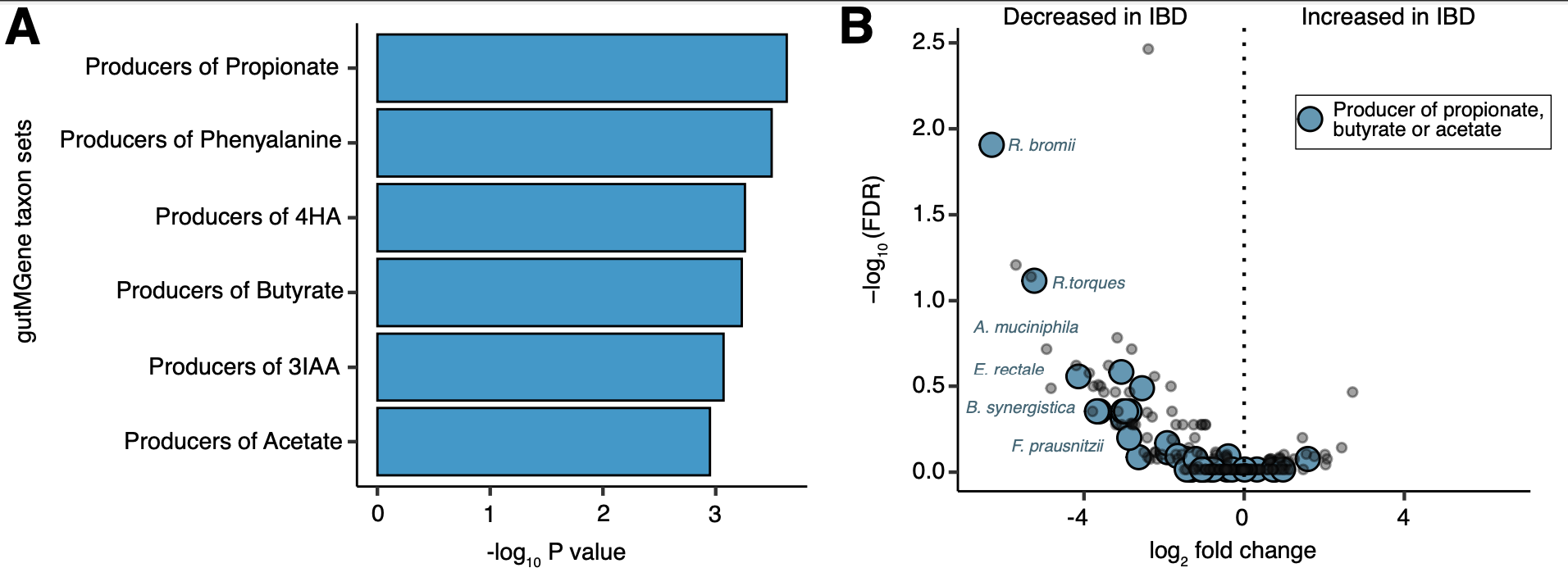
The results above were generated by using TaxSEA on the output of a differential abundance analysis comparing between disease and control. The input was per species log2 fold changes between taxa in Inflammatory Bowel disease and control. TaxSEA identified a significant depletion in the producers of certain short chain fatty acids. Using barplots we can show the overall signatures identified as significantly different. We can then highlight the individual species contributing to this signature on a volcano plot.
BugSigDB
The format of BugSigDB is that each publication is entered as a “Study”, and within this there is different experiments and signatures. For example one of the signatures may be taxa increased in an experiment, and another signature is taxa that are decreased. Users can find out more by querying the BugSigDB. In recent updates BugSigDB has moved to using the PubMed ID as the study ID (Although not all studies have these yet). See below for an example.
library(bugsigdbr) #This package is installable via Bioconductor
bsdb <- importBugSigDB() #Import database

#E.g. if the BugSigDB identifier you found enriched was bsdb:11/1/1
#This is Study 11, Experiment 1, Signature 1
bsdb[bsdb$Study=="Study 11" &
     bsdb$Experiment=="Experiment 1" &
     bsdb$Signature=="Signature 1",]
TaxSEA database with other enrichment tools
The TaxSEA function by default uses the Kolmogorov Smirnov test and the original idea was inspired by gene set enrichment analyses from RNASeq. Should users wish to use an alternative gene set enrichment analysis tool the database is formatted in such a way that should be possible. See below for an example with fast gene set enrichment analysis (fgsea).
library(fgsea) #This package is installable via Bioconductor
data(TaxSEA_DB)
#Convert input names to NCBI taxon ids
names(TaxSEA_test_data) = get_ncbi_taxon_ids(names(TaxSEA_test_data))
TaxSEA_test_data = TaxSEA_test_data[!is.na(names(TaxSEA_test_data))]

#Run fgsea
fgsea_results <- fgsea(TaxSEA_db, TaxSEA_test_data, minSize=5, maxSize=500)